
Keenan Viney
Introduction
With the implementation and subsequent repeal of the Harmonized Sales Tax (HST) in British Columbia, the debate surrounding value-added taxes is far from settled. British Columbia implemented the HST in 2010 and proponents claimed that the new tax would be more efficient than the old Provincial Sales Tax (PST). The HST would thereby make citizens better off by delivering lower prices and more jobs. However, detractors claimed that the new HST would squeeze family budgets and benefit big business at the expense of the consumer. After a large-scale petition campaign, the province voted on the HST in a referendum. The HST was repealed and will be phased out in favour of the former PST system. This paper will use a comparative statics in a two sector model to examine the effects of a value added tax versus a sales tax.
Specifically, this paper will address an often overlooked aspect of a value added tax; the emphasis on taxing only final goods as opposed to intermediate and final goods. Sales taxes like the PST, tax traded goods in each stage of the production process. For example, a logging firm would have a sales tax imposed on raw log sales to a mill. There would then be another tax imposed on the lumber that the mill sells to a consumer.
This contrasts with a value added tax which would tax only the final good, in this example, just the lumber bought by the consumer. Effectively the sales tax would be taxing the two-stage product more than a product which needs only a single level of production. This means that the cost of a good with more upgrading is greater than a good with less upgrading under a PST system. Consumers will tend to substitute away from the higher priced goods and the economy will now have a structural distortion which penalized adding value to products. One advantage of a value added tax is that, by taxing only final goods, it is neutral in its effect on the level of upgrading. Using the previous example, if raw logs are being sold directly to consumers, the imposition of a value added tax may make it worthwhile for a milling firm to open up since the tax has eliminated the premium that upgrading normally costs.
The distortion created by taxing intermediate goods may also have consequences on the size of firms. The government revenue from a tax on intermediate goods could be captured by two firms integrating vertically. For example, if the ore produced by a mining firm is taxed by a sales tax, the mining firm would be incentivized to merge with a smelting firm and capture what were previously government revenues. So, this distortion may lead to industries that are highly vertically integrated, so that all steps of a production process are carried out by a small number of large firms. Even ignoring the loss of social surplus generally associated with market power, vertical integration may make for more unstable firms. Consider a coastal town with a fishing fleet and a fish cannery. Under a sales tax these two production processes would be vertically integrated into a single firm. If the local fish harvest is poor one year, the fishery will catch little and there will be little to can. This means a bad year could put the entire integrated firm out of business. However, if the two production processes were separate, a bad year would still hurt the fishery but the cannery might well be able to buy raw fish from other regional fisheries firms. What this example illustrates is that it is important to think about the industry structure that would result from the imposition of a sales versus a value-added tax system.
Diagrammatic Analysis
These graphs contrast the effect of a sales tax with a value added tax. The sales tax is applied in much the same way as the PST, in that, intermediate goods have tax levied on them. In contrast, the value added tax is applied only to the finished goods market, much like the HST. At first glance it is easy to see that the sales tax will have a greater amount of dead weight loss, which is represented by the shaded triangles (consult appended diagram).
Part of this comes from the fact that the sales tax is collecting a higher total revenue out of the two markets. Even if the revenues were equated between the two taxes this result will still hold under certain conditions. If the intermediate good market is characterized by greater price elasticity that the final goods market, a sales tax will have a greater dead weight loss per dollar of revenue collected. Making the assumption that the intermediate goods market is more price elastic than the final goods market is reasonable if we consider budget share and substitution possibilities. For the milling firm it is quite natural to think that raw logs would make up a large share of their budgetary expenditure. Because intermediate goods take up a large portion of the budget this will mean an increase in price, through the imposition of a tax, will have a large income effect which means the intermediate goods market will be more price elastic. This is not an income effect; rather it is that price elasticity is a function of budget size. The same argument is made in labour economics where it is assumed that airline pilots will have relatively large amount of bargaining power because their wages make up a small proportion of the airlines operating budget. Another possible reason for the intermediate market to be relatively more price elastic than the final goods market is the substitution possibilities. Again, it seems reasonable to assume that there would be greater substitution possibilities for an upgrading firm than for consumers. In the case of logging, firms operating in BC will ship raw logs directly to China rather than milling them in the province. For consumers it may be possible to build homes utilizing concrete as the primary structural material. For firms that are further upgrading, substitution may be more difficult. For instance, a guitar made of concrete is both acoustically suspect and heavily impractical. To extend this thought further it is a reasonable argumentative terminus to say that the example above shows that much of the distortion of a sales tax falls on upgrading firms.
This same graph also leads to some statement about the effects of a value added tax versus a sales tax on industrial organization. As previously stated, when intermediate goods are taxed there will be fewer final goods produced. But it is possible for firms to avoid a sales tax on intermediate goods through vertical integration.
By firms merging together between intermediate markets, for instance the logging firm merging with a milling firm, the resultant company no longer has to enter into the intermediate good market. The surplus that is captured by this vertical integration is equal to the tax expenditure as well as the potential dead weight loss had the firms not merged. This incentive to merge will occur whenever there is a tax on intermediate goods and the incentive increases as the tax increases.
Also, it should be noted that the price elasticity in the intermediate goods market has a role to play in the incentive to vertically integrate. Since the intermediate goods markets may very well have greater price elasticity than the final goods market. This means that there would be greater dead weight loss for the intermediate goods market, the result of which is a sort of multiplier on the structural distortion that a sales tax causes.
However, unlike the discussion of the marginal excess tax burden, it is not possible to assess the efficiency loss associated with firms vertically integrating. What can be said is that the vertical integration is the result of distortions from the sales tax and there are some reasons why this integration may be undesirable. Firstly, integration that is spurred by a new tax is integration that that is not the result of economies of scale or else it would have already occurred. The two firms had operated separate more efficiently, and only through the distortion of the tax is a merger now marginally profitable. Secondly, there are onetime costs to integration such as setting up a head quarters and restructuring employees.
There are also persistent costs, such as greater expenditure on managerial and coordination expertise consistent with running a larger firm. Finally, there is a risk that the costs imposed by integration may be erroneous if the tax is repealed or the rate changes dramatically. Since real world firms tend to operate on a margin basis, one would assume that the imposition of tax would be followed by vertical integration with a lag of some years. This is because the firm will take some losses in the short term while searching for a firm to merge with and while hedging against a reversal in policy.
Data
The data used in the following graphs was taken from the CANSIM website and is based on the Annual Survey of Manufacturing and Logging. It should be noted that this form of the survey is relatively new having been introduced in 2004, since this is after the introduction of the HST in the Atlantic Provinces, corresponding terminated series had to be used for pre-2003 data. Care was taken to ensure that the combining of series was appropriate given the same data collection approaches were used.
This particular survey is extremely useful because unlike many of the service sector surveys it is broken down by province allowing for comparison. Furthermore, the data could have been sorted down to the industry level which is the case for the logging data. And because the logging data represents a relatively small industry for the Atlantic Provinces, it was deemed necessary to also examine aggregate of total manufacturing. This larger aggregate measure collects data from all types of manufacturing firms, from pet food producers to automobile manufacturers.
The two variables that were examined were the value added by the industry and the number of firms in the industry. Unfortunately, there is a major data gap for the number of firms in the logging industry which necessitates its removal; the manufacturing aggregate does not have this gap.
Data Analysis
Logging value added
| Summary Statistics | ||
|---|---|---|
| Atlantic Provinces | ||
| Mean | Variance | |
| 1991-1998 Growth Rates | -2.1 | 15.0 |
| 1999-2009 Growth Rates | 2.8 | 15.9 |
| Canada excluding NB, NS, NL | ||
| Mean | Variance | |
| 1991-1998 Growth Rates | 5.0 | 10.2 |
| 1999-2009 Growth Rates | -0.7 | 19.2 |
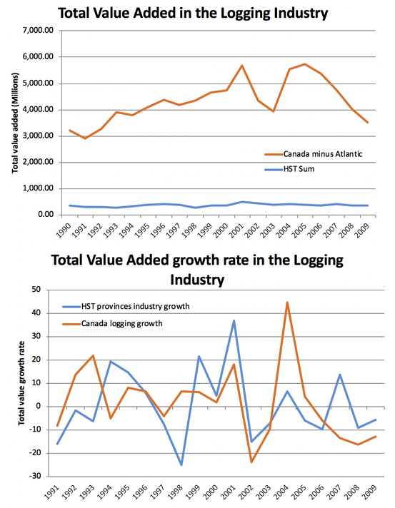
Beginning with the data from the logging industry, which considers the value added by the industry. Newfoundland and Labrador, New Brunswick, and Nova Scotia all implemented a harmonized sales tax in 1998 which effectively removed tax on intermediate goods. This change would be expected to result in a greater value added to goods given that refining has become relatively cheaper.
The summary statistics show that the mean growth in value added has increased in the Atlantic Provinces by just over four percent since the harmonized sales tax was implemented. Over the same period the growth in value add by the rest of the Canadian logging industry fell by over five percent. From the simple time series graph it is apparent that the Atlantic region adds a relatively small amount of logging value to the economy relative to the rest of the country. Considering the graph of growth rates it is evident that there is quite a bit of noise in the data which may be decreasing the accuracy of the results. Also, from the summary statistics one can see that the variance in the Atlantic region has remained stable before and after the tax giving some indication that the data was not affected by some other shock since the tax would not be predicted to change the variance. The data for the rest of Canada however, had a large increase in variance which would be associated with other shocks happening in the country. Finally, examining the three Atlantic Provinces separately, it is obvious that the value added in the logging sector is moving together across provinces. Also assuming that there would be some lag between the implementation of the HST and an effect on value added, this graph suggests that there was, at best, a small benefit due to the policy change.

Manufacturing value added
| Summary Statistics | ||
|---|---|---|
| Atlantic Provinces | ||
| Mean | Variance | |
| 1991-1998 Growth Rates | -2.1 | 15.0 |
| 1999-2009 Growth Rates | 2.8 | 15.9 |
| Canada excluding NB, NS, NL | ||
| Mean | Variance | |
| 1991-1998 Growth Rates | 5.0 | 10.2 |
| 1999-2009 Growth Rates | -0.7 | 19.2 |
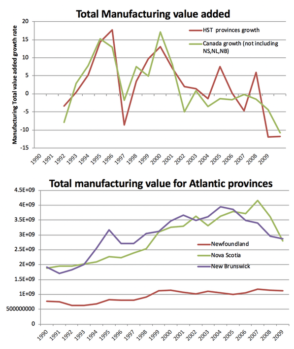
Now looking at the wider aggregate data for the manufacturing industry it is immediately apparent that there was a decrease in the growth of value added for the entire country including the Atlantic region. From the table of summary statistics it is clear that the variance in the value added growth has remained essentially constant, this suggests that the change in mean growth is primarily driven by the change in tax which should not have changed the variance.
As the growth in the value added by the manufacturing sector has slackened over the last twenty years the removal of the tax on intermediate goods has not shown significant benefit. This is in contrast with the findings in the logging industry which showed that there has been a marked increase in the growth of value added as a result of the tax. Because this is a wider aggregation it would be expected to yield a stronger result since shocks to one industry might well offset at the sector level. One issue is that financial seize up which hit the manufacturing sector hard, the graph of value added growth shows that the recession has been instrumental in bringing the average growth rates close to one another.
Before the current recession began, the graph does show that after the tax on intermediate goods was removed, the Atlantic region was generally growing value added at a higher rate than the rest of the country. Finally, the total manufacturing value added between the Atlantic Provinces shows that the tax change had a small effect. Since it seems reasonable that there would be an affective lag once the HST was implemented the final graph does seem to show an uptick in the value being added by the Atlantic Provinces in 2000. This final graph also importantly shows that the value added between provinces is moving together. This correlation is expected from the theoretic discussion previous but this graph is useful to show that an increase is driven in part by all of the Atlantic Provinces which adds credence to the argument that the tax change would have a positive effect across all of the provinces that enacted the HST.
Number of manufacturing firms
| Summary Statistics | ||
|---|---|---|
| Atlantic Provinces | ||
| Mean | Variance | |
| 1991-1998 Growth Rates | -2.1 | 15.0 |
| 1999-2009 Growth Rates | 2.8 | 15.9 |
| Canada excluding NB, NS, NL | ||
| Mean | Variance | |
| 1991-1998 Growth Rates | 5.0 | 10.2 |
| 1999-2009 Growth Rates | -0.7 | 19.2 |
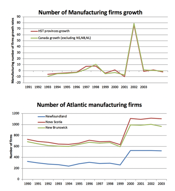
This data set had the fewest observations and also had a massive confounding event. The variance between the Atlantic region and the rest of Canada are similar which is reasonable as the change in the tax is not expected to change the growth in the number of firms.
The average growth rates seem to suggest, at first glance, that the move to harmonized sales tax actually decreased the growth in number of firms for the Atlantic region. Though this is true when looking at the summary statistics, the graph of growth rates tells a different story. In the year 2000, there was an enormous increase in the number of firms being created.
Going back to the raw data, this increase happened for each of the Atlantic Provinces as well as the rest of Canada. Upon seeing this spike one might assume that it is the result of an inappropriate data splice but this data was not spliced and was downloaded as a single data set from CANSIM.
Even more curious is that while the number of firms was exploding the value added by the industry was not spiking in a similar manner. The same spike can be seen in the graph where the number of firms is in the Atlantic Provinces are separated. It would again seem at first glance that the change in the HST has vastly increased the number of firms in the Atlantic Provinces. Since in the previous graph the spike shows up in the Canada data as well, the spike in the Atlantic Provinces cannot reasonably be driven by the HST. Because of the unknown shock that increased the rate of firm creation in this period it would be with little confidence that any conclusion could be drawn as to the effectiveness of the harmonized sales tax.
Economic Model
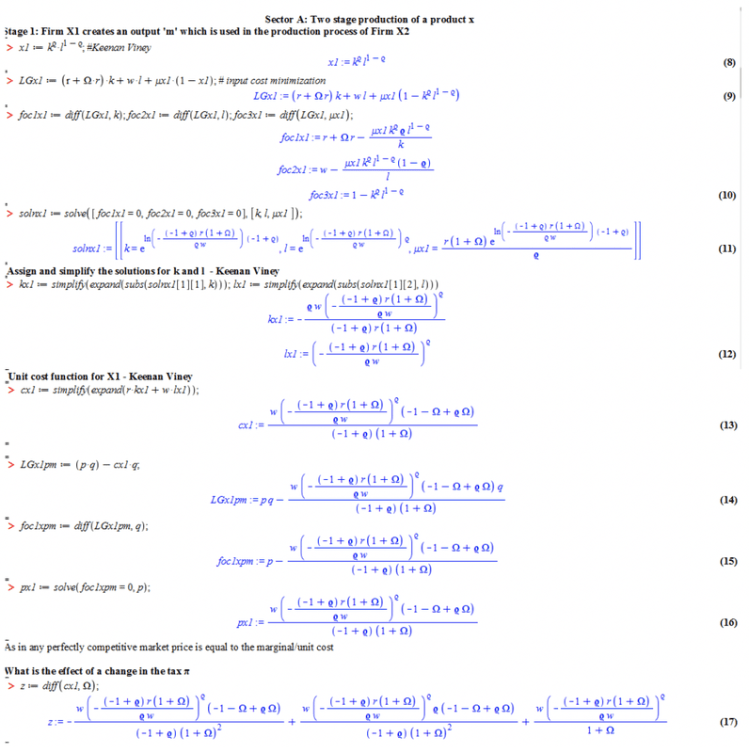
In order to address the differences between a value-added tax and a sales tax, some structure of production had to be specified. Although it would have been nice to have a closed general equilibrium model, the complicated nature of this problem dictated the use of comparative statics. The Copeland-Taylor model was considered in order to think about how firms make choices in different sectors. There were two sectors in my economy, sector B which produced good Y and sector A which had two firms producing goods X1 and X2.
Sector B operates in similar way to what would be taught in an intermediate microeconomics course. Firm Y starts by choosing inputs given a Cobb-Douglas production function. The firm minimizes the costs of inputs in producing Y, which gives us the marginal cost. Throughout this model we assume perfect competition so the marginal cost of production is equal to the price of Y. When taxes are imposed, they are on the capital input of the firm which means that the firm will substitute towards labour.
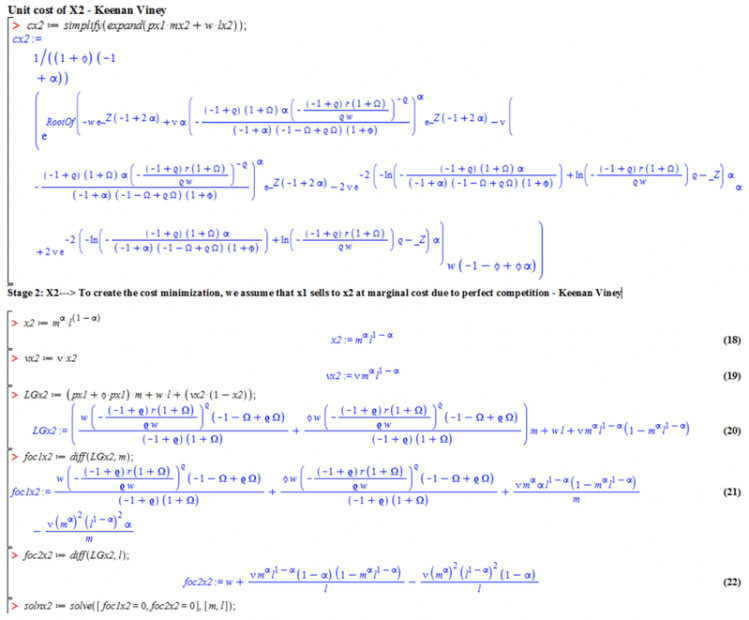
Importantly, it is the outcomes in sector A that are of interest in addressing the tax question and sector B is essentially used as a control. The A sector works as follows; firm X1 chooses its factor inputs capital and labour given a Cobb-Douglas production function and tax on capital. By cost minimizing it is possible to find the marginal cost of production which in this perfectly competitive market is equal to the price. Firm X2 then choose factor inputs labour and materials, give a wage rate and the price of X1 which is the material input. The material input ‘M’ may also be taxed and firm X2 minimizes costs to arrive at a marginal cost.
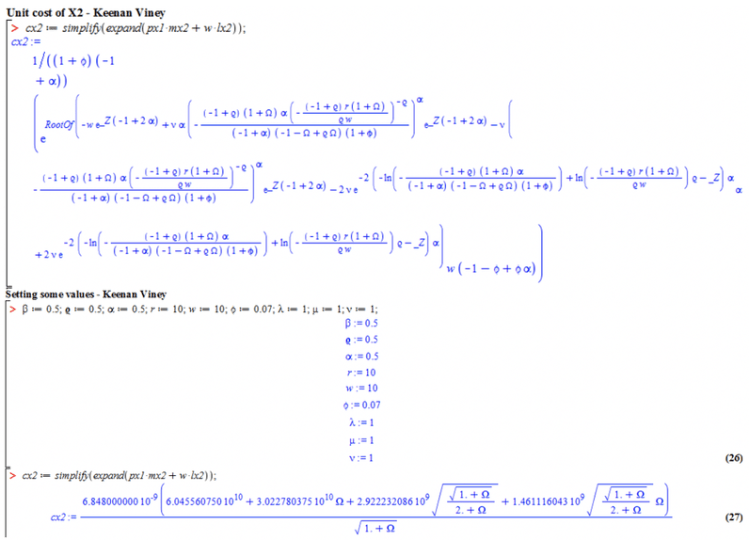
The model is first constructed without taxes for simplicity and then the taxes are added in as follows. A final goods tax is imposed on the capital inputs used in the production of Y this tax may be referred to as τ. An intermediate goods tax is imposed on the capital inputs for the X1 firm in an equivalent manor to what was done for firm Y, this tax is referred to as Ω or ω. Finally, a final goods tax ϕ is imposed on the material input of firm X2, of course because the material input is X1, the intermediate goods tax will also enter firm X2’s cost function.
Now it should be noted that the economic model above is essentially placing a tax on capital or material inputs which might be construed as something different than what a sales tax does. In fact, because sales and wage tax are considered separate by policy makers, this model captures the changes in relative price between capital and labour that result from changes in the sales tax.
Computational Method
This paper utilized the sixteenth version of Maple to work through the algebra of this model. Once the initial model was set up, the graphing and solving functions of Maple allowed for comparative statics to be used in the analysis. The graphs generated by Maple were very useful because of the complicated nature of the model. The envelope theorem was impractical for analysis and a visual representation allowed for results to be signed and visualized.
One of the advantages of using an algebraic software package is that parameters can be left unspecified throughout the model building process. When doing this type of work by hand it is necessary to assume values at the beginning of the analysis so that the algebra does not become intractable. The disadvantage to making these assumptions, and something that using Maple avoids, is the early removal of possible experiments because specified values cannot be recovered. Retaining unspecified parameters is important to any modelling if it is to investigate interactions between variables and have testable assumptions.
Experiments
This paper uses the economic model to do three experiments which will help explore the consequences and relationships between final and intermediate taxes.
Experiment 1 is meant to show that a final goods tax is equivalent to an intermediate goods tax if the firms are at the first level of production. From the economic model the firm producing Y is the first and final producer of good Y, and firm X1 is the first step in the production of good X2.
Experiment 2 examines the cost function of good X2 as the intermediate tax Ω is raised or as the final goods tax ϕ is raised. Because the intermediate tax is levied on X1 which is a material input into the production of X2, this tax enters the cost function of firm X2 in a different way than the final goods tax. The expected outcome is that the intermediate tax will have a non-linear effect on the cost function because any tax on an input into X2’s production process will be double taxed by the final goods tax. Ultimately, an intermediate goods tax will be compounded by higher levels of the final goods tax.
Finally, Experiment 3 will test what the effect of changes in the final goods tax on X2 is under of two different tax regimes. The first sets the intermediate tax to zero, which would be consistent with the HST. The second treatment has the omega value, which is the intermediate goods tax, equal to the final goods tax which is similar to what would occur under the PST.
Results
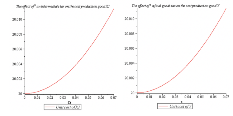
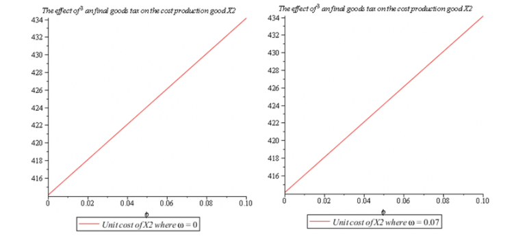
Experiment 1: Shows that the effect of an intermediate tax on X1 and a final tax on Y.

As expected, the change in cost that results from taxing product X1 and Y are symmetric. For a tax rate between zero and 7%, both graphs show an increasing cost that results from the tax Ω on X1 and the tax τ on Y. This result is not surprising since with respect to the firm producing X1 the intermediate tax Ω is no different than a final tax. Though the result is not a revelation, it shows that the cost function of X1 is working in the same way as that of good Y which will make the results in the next experiments more convincing.
Experiment 2: Compares the effect on the unit cost of X2 when the intermediate and final goods taxes are changed.
These graphs compare the change in cost of production associated with a change in either the intermediate tax imposed on the capital input of X1 or the final goods tax that is levied on the material input in the production of X2. The most striking result is that the intermediate goods tax omega, increase costs in a non-linear manner. This is due to the fact that an intermediate tax increases the price of X1 which increase the price and associated tax on good X2. This contrasts with the final goods tax, phi, on the cost of X2 which is linear. This linearity arises from the fact that the final goods tax does not compound the effect of an intermediate tax; the next experiment will show that a final goods tax is independent of the intermediate tax.
Experiment 3: Examines the dependence of Firm X2’s cost function on the final goods tax under two different intermediate goods tax regimes.
This experiment shows that changes to the final goods tax are independent of the tax rate on X1. This result may seem surprising, given that the previous experiment showed compounding of the intermediate tax on the cost function of X2. It is important to remember that the specification of this model is that the producers are operating in perfectly competitive market. By taking the price of inputs as given the intermediate tax on material inputs for good X1 is endogenized within the firm producing good X2.
Discussion
This paper has shown that taxing intermediate goods has a distinctly different outcome than when only final goods are taxed. This result is something that was largely ignored in the British Columbian debate over the efficacy of the HST. By taxing the intermediate goods a perverse incentive is created whereby adding value is penalized. The often heard rhetoric of resources being shipped away without upgrading has lead to slogan that suggest bans on raw log exports. But few would point to the tax system as a possible source of the incentive firms have to export resources raw. The non-linearity of intermediate goods taxes on the final cost of production seems to suggest that the PST may be a conspicuous culprit.
One of the limitations of this analysis is that it does not use a full general equilibrium model. This does not properly allow for the analysis of welfare loss or the substitution effect on labour that the tax systems would give rise to. The problem with using a more extensive model is the added complication associated with the functional forms. Where in a single firm example it is possible to utilize the envelope theorem for many modes of analysis, the addition of another firm ruled this out as the functions quickly became intractable. A general equilibrium model would only have served to increase this problem.
Another limitation of this analysis is that it does not take into consideration the level of government revenue under the different tax systems. This was done because it makes the analysis more externally valid to the situation in British Columbia. Taxing a greater number of goods under the PST should raise more revenue for the government. To make the transition between tax systems revenue neutral the HST tax would have to be at a higher rate since it taxes fewer goods. However this is not what happened in the province, both the PST and HST were seven percent and this is incorporated into the assumptions used in this paper, always setting taxes of either the final or intermediate goods tax to seven percent.
Appendix
Data sources
Logging value added data series from 1990-2003: v1408462, v1408465, v1408686, v1408688, v1408702, v1408704, v1408705, v1408926, v1408928, v1408929, v1408941, v1408955
Logging value added data series from 2004-2009: v41339407, v41886162, v41886181, v41886187, v41886190, v41886248, v41886267, v41886276
Manufacturing number of establishments data series from 1990-2003: v761791, v761793, v761795, v761796
Manufacturing number of establishments data series from 2004-2009: v41552914, v41564561, v41566494, v41568016
Manufacturing value added data series from 1990-2003:v762029, v762031, v762033, v762034
Manufacturing value added data series from 2003-2009: v41554669, v41565382, v41567637, v41569172
References
Annual survey of manufactures and logging (asml). (2011, August 4).
Retrieved from http://www.statcan.gc.ca/cgi-bin/
imdb/p2SV.pl?Function=getSurve
y&SDDS=2103&lang=en&
db=imdb&adm=8&dis=2
Frank, R & Parker, I . 2007. Microeconomics and Behavior. Toronto: McGraw-Hill.
