
Keenan Viney
Abstract:
Expectations play a vital role in the current approach to macroeconomic modeling. By studying the role of expectations directly, it is possible to gain insight into how the economy aggregates and utilizes information. This paper examines whether or not expectations themselves can drive real output. The results suggest that in Canada, expectations are not self-fulfilling and are simply the best forecast of agents about the future. Additionally, better predictions about the future have not made output less variable.
I. Introduction
Within the real business cycle (RBC) literature, expectations have always been important when modeling rational agents who are forward-looking. Any economic shock will cause changes across many periods which are optimally anticipated by an agent.
A new avenue of study in RBC models was opened by Jiamovich and Rebelo who suggested that the anticipation of coming real productivity shocks could explain a large portion of the business cycle (2009). These ‘news shocks’ are similar to the ones generated by the Solow residual and are key to understanding early RBC frameworks in which a positive shock increases aggregate productivity. The difference is that news shocks are set to occur with uncertainty sometime in the future, so that an agent knows, for example, total productivity will be higher in the next month while current productivity remains unchanged. The distinction between these two shocks allows for Jiamovich and Rebelo to argue that it is the expectation of shocks which can lead to real volatility.
This also suggests that business confidence surveys may have an important role in predicting future output and also the anticipation of coming shocks can make forward-looking agents change their current behaviour. Another feature of news shocks is that the news of coming increased productivity may turn out to be false and this can cause a recession. It follows then that more accurate forecasts of future economic activity can moderate the business cycle. Jiamovich and Rebelo suggest that better predictions about whether news shocks will actually result in an increase in productivity was an important factor in the ‘great moderation’ observed in macroeconomic aggregate variables through the 1990’s.
By using a monthly tri-variate structural vector auto-regression this paper will examine the relationship between output and business sentiment. Not only should business sentiment be able to predict future output, as we would expect in a rational expectations framework, but there may also be another channel of expectations.
There are two distinct views of expectations in the business cycle. The first has already been discussed; that business sentiment should predicted changes in output for the economy, this is known as the news view. The other channel of expectations is similar to what Keynes thought of as animal spirits, this is the notion that sentiment itself can cause changes in output. For example, it may be that positive business sentiment based on no observable economic fundamentals causes firms to increase their investment and production; this is the animal spirits view.
The animal spirits view is often contentious in that it prescribes real effects to apparently non-rational behaviour. However, there may be argument for the additional study of animal spirits. The seminal contribution of Diamond (1982) to search theory suggested a view of the macro-economy that was characterized by multiple equilibria for the total output of the economy. There were equilibria where there were high levels of productivity, characterized in the Robinson Crusoe imagery, of agents willing to climb very high trees, at great cost, to produce a large supply of coconuts. A macro-economy could also get caught in a low output equilibrium, which is interesting in a development context. Although there is great persistence in output among developed countries, it is possible that expectations are the avenue to move between equilibria of different output levels. Said another way, Diamond’s search model implies that many different output levels can be sustained, despite not knowing the exact origin of the animal spirits, the relative pessimism or optimism agents may cause some of the fluctuations in output which we observe.
The policy implications of this paper focus on how best to moderate the business cycle. Following the financial crisis in 2008, many explanations for the great moderation were thrown into question. If it is true that better prediction can itself moderate the business cycle as Jiamovich and Rebelo (2009) suggest, then the recession should stand out as a period where expectations were not well formed. If animal spirits are important to the Canadian economy their source should be explored. Fundamentally, intellectual curiosity cannot ignore a driving process of the Canadian economy[1]. More importantly, understanding macroeconomic fluctuations is important because they have real welfare consequences. Although consumption is smooth across the business cycle, there are large variations in employment which are not equally distributed across the population. This paper will help to further understanding of the driving process of the business cycle in Canada.
The rest of the paper is organized as follows. Section II will review the literature relevant to understanding the role of expectations. Section III discusses the source of the data and displays some summary graphs. Section IV shows the VAR model used and some of the assumptions that go into its development. Section V goes through the results of the data manipulation and VAR modeling. Section VI discusses the various robustness testing of the VAR model utilized in the previous sections. Finally, Section VII concludes the paper.
II. Literature Review
The difficulty in studying expectations is well summarized in ‘Toward a Transformation in Social Knowledge’ by Kenneth Gergen. He examines the early literature on expectations which highlights the enlightenment problem whereby publishing predictive results could change agent’s behaviour and falsify the results. Game theory was the first branch to deal directly with the problem of this infinite regress by using convergence.
Another relatively early paper which emphasised the importance of expectations was the Lucas critique (1976). This paper spurred a shift in macroeconomic modelling to rely on microeconomic foundations and rational agents which together removed many ad hoc assumptions and made results robust across policy regimes.
Early business cycle models focused on contemporaneous shocks to productivity, Jiamovich and Rebelo suggested that more of the business cycle could be explained if news shocks were used as well. Rather than a technology making the economy more productive today, a news shock is the signal of future technological progress or implementation in the future which nevertheless causes agents to begin reacting today. Using news shocks allows for the possibility that an impending technological shock may turn out not to have the expected productivity effect if the innovation is a bust. An implication of this structure is that if agents can accurately predict the productivity outcome of a news shock then the volatility of macroeconomic aggregate variables would decrease. Jiamovich and Rebelo identify better predictive technology as a possible cause of the ‘great moderation’. The great moderation can be seen in a decrease in the standard derivation of United States output, hours worked, investment, and consumption from 1947-2004, using 1983 as the break point.
Output persistence has also increased over this period. Jiamovich and Rebelo do a rudimentary test of their theory of the great moderation by using the Livingston survey of unemployment forecasts. This survey is an aggregation of expert opinions on the change in unemployment at a two-quarter horizon, the sample used goes from 1961Q4 to 2003Q4. Following other literature on business cycle moderation, the authors choose a breakpoint of 1982Q4 to separate the high and low volatility period. They find that the average percentage forecast error decreased from 3.3% in the earlier high volatility period to only 1.5% in the later low volatility period; overall, forecast error declined by 79%. Of course forecasting future unemployment becomes easier if the underlying variable, unemployment, has become less volatile. However, the standard deviation of unemployment declined by only 23% across the subsamples which implies that predictive capacity has increased by 56% and given the theory of news shocks, the increase in predictive power is hypothesized to play a role in the great moderation (2009).
A more thorough look at the great moderation was done by Stock and Watson in 2003. Again they focus on the US, finding moderation in output, employment, and consumption growth as well as sectoral output growth (which was an important innovation of the Jiamovich and Rebelo news shocks RBC model). Simon (2000) finds that this trend has occurred across the OECD.
For the US, moderation occurred sometime between 1983-1985 and saw a decrease in the conditional variance while there was no change in the conditional mean of output growth. The results of their multivariate VAR suggest that moderation was coming from smaller economic shocks rather than less persistence in the macroeconomy. The results are also decomposed into their sources; better macroeconomic and monetary policy account for 10-25% of the moderation, while ‘good luck’ due to commodity and price shocks account for 20-30% of the moderation. This decomposition still leaves 40-60% of the moderation unexplained and this leaves room predictive technology to be a factor. Furthermore, these explanations are less plausible after the recession which started in 2008; now is an auspicious time to further investigate whether increased predictive capacity might be smoothing the business cycle.
Stock and Watson identify the reason that moderation is desirable; reduced output volatility implies fewer and shorter recessions (2003).
The other question which this paper seeks to address is whether economic expectations can be self-fulfilling. Barsky and Sim (2010) is a recent paper which addresses this question using the Michigan survey of consumer confidence and US data. They use a tri-variate VAR and find the impulse response of consumption and income to innovations in consumer confidence. They also find that consumer confidence is not Granger-caused by income or consumption. Taken together, these two results support the animal spirits view. It seems that economic sentiment, measured by consumer confidence, is causing real economic outcomes. This contrasts with confidence surprises merely summarizing news about future economic prospects, as in the news view. The authors try to decompose the consumer confidence measure by using other responses from the Michigan survey, however this does not help explain movements in the growth of consumption or income. The authors use this to suggest that confidence surprises are not related to tangible news in the economy. However, an important critique of this paper regards the failure to include any leading macro-aggregates in the structure of the VAR. By using only a variable for consumer confidence, consumption, and income the information set is constrained which may lead to misidentification. Said another way, the equation of the VAR system which explains consumer confidence will consist of its own lagged values and the lagged values of consumption and income. Of course we would not expect this equation to fully capture how consumer confidence is determined but if important variables are omitted then the shock that is generated by a confidence surprise (when the explanatory variables do not correspond to the dependent variable) is not actually a shock. If a more complete set of explanatory variables was included then more of the shocks could be explained by variation in these new variables and the innovations of the VAR model would look different. In the Barksky and Sims paper there is no inclusion of a leading macroeconomic variable. Since consumer confidence is forward-looking, it seems odd to not include a macroeconomic variable that predicts the future, and presumably is an indicator that forward-looking agents use when responding to the consumer confidence survey. Another problem with the methodology of this paper arises from the structure of the survey data, the following two papers address this.
In Grisse (2008) German output is used along with a leading indicator and a survey of business confidence to investigate whether expectations are self-fulfilling. The key difference with this paper to Barksky and Sims is that contemporaneous restrictions are dropped in favour identification through heteroskedasticity. Grisse’s argument for this is that not allowing for contemporaneous correlation of output and expectations could be a problem. Economic activity cannot contemporaneously effect expectations because output numbers are published after expectations are formed. However, since there are inevitably omitted variables in the information set, contemporaneous effects cannot be restricted due to systemic variation. Identification through heteroskedasticity requires designating a number of periods of high variation known as regimes. A number of non-overlapping regimes are sufficient to estimate the variance-covariance matrix which just identifies the structural form and allows for its estimation. There are two assumptions of this procedure which are immediately apparent. First, structural shocks must not be correlated, this is a common assumption made in the VAR literature, and was the reason that econometricians have moved away from reduced-form estimations which do not provide orthogonal shocks. Secondly, it is assumed that the parameters are stable across the heteroskedastic regimes. This assumption is strong and it is unclear whether it is appropriate given the particular characteristics of this problem.
When Stock and Watson (2003) examined output moderation they found that across two regimes over the past four decades moderation had come from smaller shocks rather than a decrease in shock propagation which would have shown up in different coefficient estimates across regimes. Here it is reasonable to use the assumption that coefficients are stable while it is the shock magnitudes which are changing. However, the same assumption used in Grisse’s identification strategy is less convincing because there are four different regimes derived from a relatively small sample of quarterly data. The regimes are also chosen in an ad hoc manner, not coming from regime changes identified by economic theory.
The arbitrary optimization exercise done by Grisse, the originator of this technique, Rogobon (2003), where identification is backed up by economic theory. Rogobon (2003) uses identification through heteroskedasticity to investigate the cross-country effects of Latin American sovereign debt. Because Mexican shock can contemporaneously effect Brazil, for instance, and the reverse is true, it would be inappropriate to restrict contemporaneous effects in either direction. The heteroskedastic regimes come from economic observation; crises such as the Tequila crisis, Russian default, South Asian financial crisis of 1997. These events are plausibly enlisted in identification because they are known to have affected the Latin American bond markets. Said another way, when looking at the bonds market there are obvious episodes and crisis that can be used as regimes in identification. The same argument is difficult to make for expectations and without any economic theory to support the selection of various regimes there is no glaring advantage to using a method that is significantly more computationally expensive.
A final paper which addresses issues important to this project was written by Schmitt-Grohé and Uribe. They use a dynamic stochastic general equilibrium (DSGE) model, estimated by maximum likelihood and Baysian methods, and are used to better understand the component effects and timing of news shocks (2010). This approach can capture multi-period anticipation and helps highlight a problem that is endemic to surveys of business or consumer sentiment. In a quarterly survey like the Michigan consumer confidence survey in each period there is an aggregate forecast of what conditions will be in the next year, or the next four quarters. In the next quarter, the survey now forecasts an additional quarter into the future but there has also been the realization of new fundamentals in moving to the next quarter. For example, an initial January 2000 survey would deliver an aggregate forecast of what businesses think will happen between January 2000 and January 2001. At the start of the next quarter, April 2000, there is a new forecast about what businesses think will happen between April 2000 and April 2001. Two things have changed between these two forecasts. The second forecast adds a forecast of what will happen between January 2001 and April 2001. The second forecast is also different because it is made based on additional information that was realized moving from January 2000 to April 2000. Schmitt-Grohé and Uribe’s approach attempts to untangle these two effects with some success (2010). However, this problem will be carefully addressed in this paper while staying within the parsimonious framework of a VAR.
III. Data
The data used in the models of this paper were obtained from a variety of sources. All of the models have data on Canadian output and a leading indicator index which were compiled by Statistics Canada and retrieved through CANSIM.
Output data at both a monthly and quarterly frequency is used and in all cases it is deseasonalized and represents the final data revision. The leading indicator index is an unweighted index of ten economic variables which lead output cyclically.
The 10 components of the index are money supply, TSX composite, non-agricultural employment, a leading indicator index from the United States, housing construction starts, average hours in a work week for a manufacturing worker (which proxies for labour utilization). The length by which this index leads output is variable but is not systemically related to the level of output. The index is also standardized so that its growth rate is equal to GDP; however it’s variance is higher than GDP because “the components of the index are highly sensitive to changes in aggregate demand” (Statistics Canada, 2011).
Throughout this paper the unsmoothed leading indicator index is used, in part, because more variance increases the explanatory power of the VAR model. The smoothed data set is better for making accurate forecasts of future output; however using smoothed data implicitly restricts the information available to the agents when choosing their expectations which may cause the expectations shock to be misspecified. The smoothed data set is made using a five-month moving average and Statistics Canada argues that the smoothed series provides a better signal of changes to fundamentals and reduces the impact of revisions. However, to the extent that the components of the leading indicator index enter agent’s forecasts, the data is coming in unrevised. Ideally, we would like all the data in the model to be unrevised to more accurately reflect the information available to agents when forming their expectations, unfortunately unrevised output data is not available at the monthly frequency.[2]
The main model of this paper uses the Canadian Business confidence survey as a measure of economic expectations. The Canadian Business confidence survey is conducted by the Ivey School of Business at Western and records the expected purchases of a panel of purchasing managers. The sample of purchasing managers is selected to capture both the regional and sectoral heterogeneity in the Canadian economy, as well as both the public and private sectors. This survey is similar to the German industrial production index which was used in Grisse (2008). The Ivey survey is also known as the purchasing managers index (PMI). It asks purchasing managers “Were your purchases last month higher, the same, or lower than the previous month?”(Leenders, 2013). This survey question is related to organizational activity, and in aggregate the purchasing managers are giving a proxy for expected aggregate demand which effects output. Other studies done with US data, such as Barksky and Sims (2010), use a consumer confidence survey published by Michigan State. Consumer confidence is much the same as the PMI, in that both are effectively measuring expected future aggregate demand. Using the PMI for expectations makes sense because raw material purchases will eventually make up output after upgrading. Those managers who purchase more than normal are expecting that demand will be sufficiently high to support the increased production. It is also important to note that purchasing managers have an incentive to correctly predict future demand and output in order to minimize the cost of large inventories or stock-outs. Furthermore, while individual managers may only focus on their own sector, the survey is essentially bringing together all of the various idiosyncratic expectations into an aggregate expectation variable. The PMI survey has one final feature which makes it particularly attractive to use; it is collected with a monthly frequency. This is in contrast with the following two expectations measures from the Bank of Canada which are only collected quarterly. Higher frequency data minimized the censoring problem which we will return to later in this section.
The expectations data for the two secondary models comes from the Bank of Canada. These two quarterly data sets are collected as indictors of future economic activity and both sets run from 1998Q3 to 2013Q1. The survey is drawn from a sample of 100 senior managers from across the country who are chosen to roughly replicate the composition of the Canadian economy. While the Bank of Canada tries to ensure the representation of their sample, they admit that the small sample size is undesirable. The survey asks a number of question but the two relevant to this paper are about future sales growth (FSG) and investment in machinery and equipment (IME). The question about FSG asks “Over the next 12 months the rate of increase in your firms sale volume is expected to be higher, the same, or lower compared with the last 12 months.” It should be evident that higher expected future sales are related to output through increased production. The question about IME asks “Over the next 12 months, your firm’s investment spending on machinery and equipment (compared to the previous 12 months) will be higher, the same, or lower.” (Bank of Canada, 2013) A possible connection between output and IME is provided by Greenwood et al (1992). They found that price declines in investment-specific capital, such as equipment and machinery, were able to explain a large portion of output growth in the post-WWII era. These two data sets are separately employed as expectations variables in order to generate some additional results to be compared with the main model which uses the monthly PMI. The disadvantage of the Bank of Canada data sets is that they are quarterly, and given the relatively short sample period the number of observations is low which results in imprecise estimates which are especially apparent in VAR estimation.
[1] Unlike the general apathy towards studying the underlying properties of the Solow residual
[2] An area for further research would be to use the output and leading indicator revisions as an instrument or new type of model shock to further assist in identification.
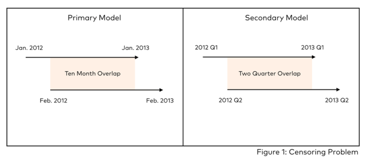
Beyond the larger sample, using the PMI as expectations is advantageous because it minimizes, what has been referred to in this paper as the censoring problem. As explained in the literature review section, two things are happening simultaneously when moving between periods in the expectational variable. With each new forecast an additional period comes into the expectation while new information is realized about the economy with the benefit of an additional period of time. Since it was not feasible with the VAR approach to separate these two effects, attention is paid to minimize the problems that arise from not using a full DSGE model. One way to address the problem is to minimize the differences in each adjacent expectation, or in other words to maximize the overlap between expectation observations. This is accomplished by relying on higher frequency data where possible.
As Figure 1 shows, monthly data overlaps itself by 10/12 while in contrast quarterly data overlaps by only 2/4. This is the main reason that we rely primarily on the PMI dataset and only use the other two quarterly data sets to discuss the validity of this papers finding.
Before moving on to the model specification, it is elucidating to examine some summary statistics and figures. The primary model, which uses PMI as the expectations variable, is over a sample from January 1999 to April 2012. Over this period the average output growth is 2.2% while the average expectation was 57.5 from a base of 50. This indicates that those surveyed in the PMI were much more optimistic about output growth than what was actually realized. The difference between the two averages could be explained by some sampling bias which generally skews responses in an optimistic direction. This is not a problem for the identification in the VAR model.
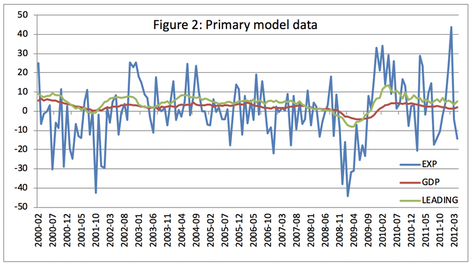
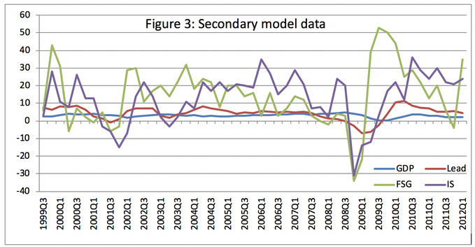
Figures 2 and 3 show the plotted variables of the primary and secondary models. It is immediately apparent that in both summary, figures output has much less variance compared to other variables in these models. The leading indicator index is more variable than output due to its construction. All of the expectations variables; PMI, IME, and FSG have high varian
ce relative to output but have broadly similar patterns, leading cyclic changes in output growth. The high variance of the expectations variables is coming from the same mechanism that makes asset price volatile: new information changes expectations at a number of time horizons which causes large movements in the expectations variable because it is aggregating expectations across 12 months. In the context of the primary model, an unexpected output revelation in a single month may have implications for expected output at 3, 5, and 9 months in the future, for example. Since the expectation is for the coming 12 months if all three of these time horizons have downward revisions then there will be a large drop in the next months expectation.
IV.Model
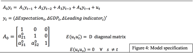
The equations and matrix shown in Figure 4 represents the primary VAR model estimated by this paper. The vector yt houses all of the endogenous variable used in the models; expectations, output, leading indicators. When yt is post-multiplied by the A0 matrix, its recursive structure results in a product which exactly-identifies the equations, ordering the variables from most exogenous to least exogenous.
The ordering of expectations first, output second, and the leading indicator third follows Barksky and Sims (2010). Expectations are set as the most exogenous variable in all specifications because it is observed before the other two variables are published. For example, the expectation for February is surveyed in January and hence the output and leading indicator in February will not be able to affect the expectation variable contemporaneously. Said another way, expectations do not depend contemporaneously on any other variables and so, expectations are explained by the lag of output and the leading indicator (which has information about future output) and the lag of expectation. Output is ordered second and the leading indicator is ordered last because a low leading indicator value would not directly impact output in the same month as the leading indicator provides information about future output. These model restrictions allow for orthogonal shocks but because they are imposed prior to estimation, the restrictions are not testable.[1]
The main innovation of this model compared to the past literature is the use of the leading indicator index. This variable is included because it would be in the information set of the survey respondents. In the case of the PMI, purchasing managers have an incentive to pay close attention to variables which lead output and signal the future level of aggregate demand. By not including a leading indicator, other authors have effectively added changes in future economic fundamentals, as captured by the leading indicator, into the expectations shock. In doing this, it becomes unclear whether an unbridled optimism of animal spirits has lead to an increase in output or if it was simply that there were signals present of impending auspicious economic times. Without including the leading indicator in the model the two causes would have an indistinguishable effect.
V. Results
Before delving into the results from the VAR models, we will first address the predictive technology thesis of Jiamovich and Rebelo. They argued that much of the business cycle could be explained by news shocks. These shocks are similar to the total factor productivity shocks generated by the Solow residual except that agents know with some uncertainty that the shock will come several periods in the future as opposed to immediately.
After modeling these shocks Jiamovich and Rebelo suggest that if an economy could better predict the outcome of news shocks, the economy would display lower output variance. The statistics which Jiamovich and Rebelo show are related to US unemployment numbers, they show a decrease in the variance of both the expectations variable and output, the former being relatively larger implying that prediction had become better[2]. Since news shocks can be moderated by better prediction, this informal example was suggested to be reason for the ‘great moderation’ in macroeconomic aggregate data in the 1990’s (2009). We now realize that the ‘great moderation’ was a transitory phenomenon but the proposal of Jiamovich and Rebelo may still hold if there has been technical regress in prediction.
Canadian data suggests that predictive accuracy cannot explain changes in the standard deviation of output. Using monthly output data and the PMI survey, then separating the series at the midpoint, the subsample standard deviations can be calculated. From February 1999 to May 2005 the standard deviation of output was 1.45, from June 2005 to April 2012 this increase to 2.27, a change of 56.9%. The standard deviation of the PMI survey is 13.39 in the first period and 16.27 in the later period, an increase of 12.61%. So, output variance increased as did the variance of expectations though to a lesser extent. Of course, we would expect the variance of expectations to increase if output, the fundamental on which the expectation is being formed, is increasing. However, for the theory of Jiamovich and Rebelo to hold we would need to see an increase in the PMI survey variance be greater than the increase in output variance, this would suggest the predictive regress. The gap between the two changes in standard deviation is 44.3%, this increases to 55.3% when the breakpoint is moved closer to the 2008 financial crisis, specifically April 2007. Using the Bank of Canada survey and using IME and FSG as proxies for expectations yields similar results which appear to contradict Jiamovich and Rebelo’s claim that predictive technology is an important factor in moderating output fluctuations.
[1] Other plausible orderings were estimated and the results are not sensitive to this change. However, this is not a true test of these restrictions since it involves using results from misspecified models.
[2] See Section II
Now moving to the VAR model it is possible to further explore the relationship between output and expectations. The results in this paper are contrary to many other findings which claim ‘animal spirits’ have an influence on output.
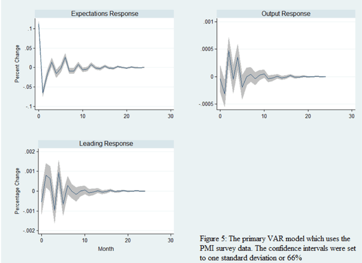
Figure 5 shows the impulse response of all three variables; expectations from the PMI, output growth, and leading indicator index growth, to a positive one standard deviation shock to expectations. A shock to expectations occurs in the model when expectations are not explained by the dynamic structure of the expectations equation. The first element of these graphs to note is that the y-axis differs between graphs. This was necessitated by the fact that, as in many VARs, shocks mainly affect their own variables which will be explored further in the forecast error variance decomposition (FEVD).
Figure 5’s first panel shows that the expectation response to a shock of unexpected optimism is a large negative correction in the first and second months after the shock, followed by statistically significant oscillation around the long-run value from months 3-8 excluding the 5th month. The implication of this result is that when expectations are optimistic, beyond what can be explained by the elements of expectations own explanatory variables, in the next period there will be a more pessimistic expectation than would have been predicted. After this point, the coming months will see relatively small but statistically significant bouts of pessimism and optimism as a result of the onetime expectations shock. More interesting still is the effect of the unexpected positive expectations shock on output. The initial response is small and negative but in months 2 and 4 there is a statistically significant positive response of output. Since the confidence intervals are set to one standard deviation (66%), the statistical significance of the output response to the expectation shock is marginal. Furthermore, despite the statistical significance of the output growth response, at no point is the response economically significant; the absolute upper bound of the response is a 0.0007% increase in economic output growth in two month after the shock.
The result from this impulse response function suggests that in Canada the news view of expectations is more important than the animal spirits view. The news view holds that expectations are simply the survey respondents’ best available prediction of future economic output growth. The muted response of output to unexpectedly optimistic expectation suggests that expectations are not self-fulfilling as in the animal spirits view.
Support of the news view contrasts to a number of related papers in the literature and it is worthwhile to consider some of the methodological differences that may contribute to this papers result. As stated, this paper follows the tri-variate methodology of Barksy and Sims with one important difference; the use of the leading indicator index in place of consumption. By using a survey variable for expectation, output, and consumption, Barksky and Sims are restricting the information available to a hypothetical agent choosing the level of the expectations variable. Said another way, we know that when agents form expectations about the future they use quite a large amount of data in aggregate. Although a single agent may only know how much raw material purchasing their own firm is doing, as in the PMI, when aggregated, the consensus view embodies a large amount of information. It seems natural to think that when forecasting the future the most important macroeconomic indicators would be the variables which lead output. By not including this relevant information, the expectations shock is being misspecified and this misspecified expectation shock causes a significant change in output IRF. In fact, Barksky and Sims effectively acknowledge this problem by pointing to the fact that output and consumption do not Granger-cause expectations in their model, they need for this to hold because if it does not, then reverse causation confounds the misspecified shock. In this paper, the model replaces consumption with the leading indicator index. The idea to use a leading variable to minimize anomalous results is not new; Sims (1992) suggested using oil prices as a leading variable to address the well known price puzzle that arises when attempting to identify monetary policy. Using the leading indicator makes the claim of the expectation shock being identified easier to make. To exclude the leading indicator is to exclude a valuable source of information about the future which is surely utilized by agents when forming expectations. The only serious draw back that using the leading indicator brings is multicollinearity. Because both the leading indicator and expectations predict output the two series move together. Multicollinearity is a particular problem in a VAR as the model is already very unrestricted which quickly decreases the available degrees of freedom. This is one explanation for the low degree of statistical significance in the IRF results but to not include the leading indicator would be to exclude a relevant regressor in favor of model parsimony.
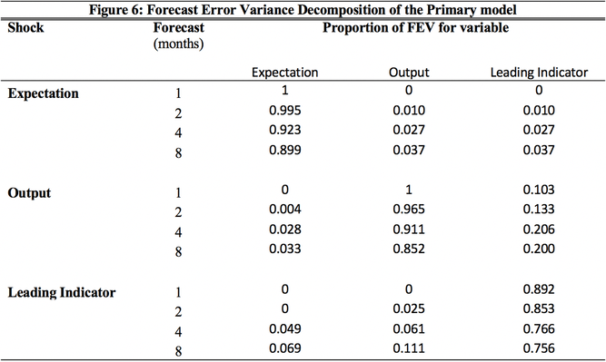
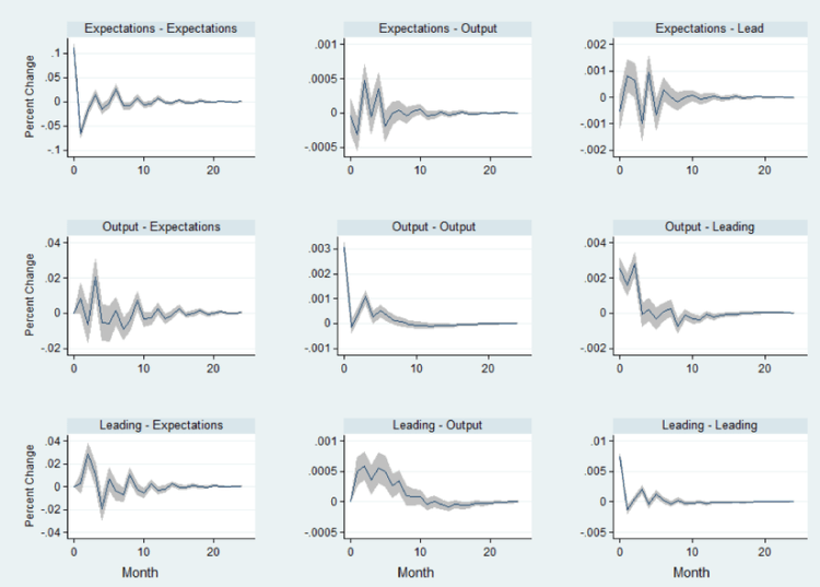
The FEVD (Figure 6) shows the relative amount of variation that a given shock contributes to the variance of an endogenous variable. By using this measure, it is possible to infer the relative importance of different shocks in determining the variance of variables used in this model. From Figure 6, it is apparent that the expectations shock is less important in explaining the variance of output than the variance of expectations themselves.
These results are consistent with the impulse response graphs in Figure 5, expectations shocks having the largest impact on the expectation variable itself. Figure 6 also delivers a result often seen in VARs which is that a variables shock mostly explains that variables variance. This can also be seen in the full set of IRFs which appears in the appendix. Finally, it should be noted that the results from the Figure 6 differ from FEVD in Barksky and Sims due to the difference in methodology but, where the two models do overlap, broadly similar results appear.
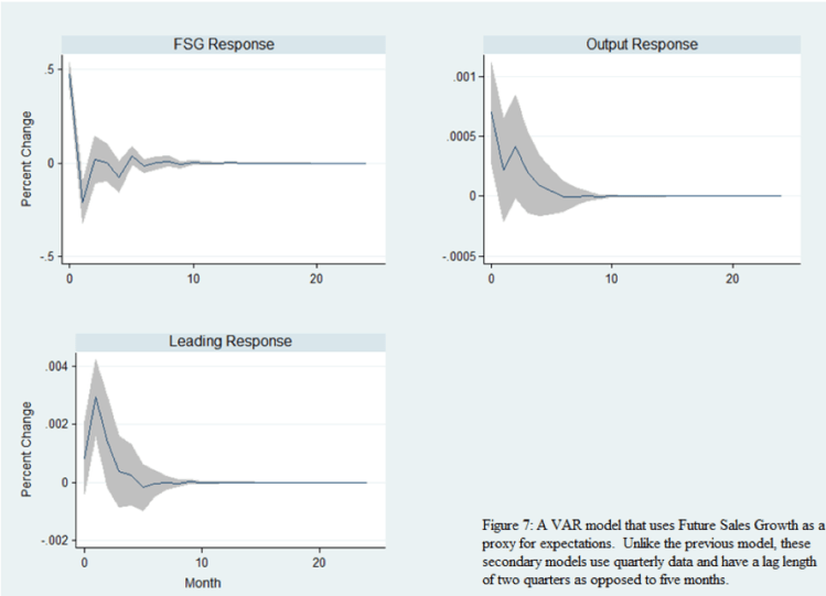
In order to ensure the generality of these results we now turn to the survey data collected by the Bank of Canada. Future sales growth and Investment in machinery and equipment are separately substituted in to a similar model structure. The main difference is that this data is quarterly and roughly the sample period so the number of expectations in low. As such, when testing was done on lag lengths a split recommendation of two and six lags, two was chosen because six lags had so few degrees of freedom that any effect would have had an extremely imprecise estimate and would have large confidence intervals. The graph in Figure 8 uses future sales growth as a proxy for expectations and shows the response of each variable to a positive one standard deviation shock in expectations (FSG). The results tend to agree with the model using the PMI survey (see Figure 6); expectations itself follows an oscillatory pattern back to steady state. Both output and the leading indicator have positive statistically significant responses, but neither are economically significant. Despite the small magnitude of the output growth response, its shape is similar to the one found by Barksky and Sims (who were also using quarterly data) this lead them to conclude that animal spirits influenced output while in Figure 7 the results contradict this.
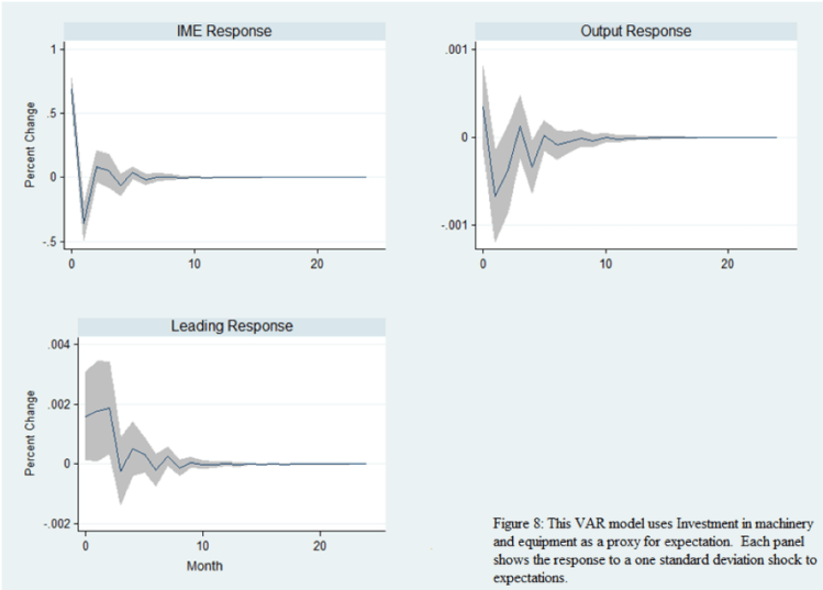
Finally, Figure 8 shows the IRFs of the model which uses investment in machinery and equipment as a proxy for expectations. Here again a similar pattern emerges. The expectations shock primarily acts on expectation themselves but of all the results using IME has the least oscillation in response to the shock.
The output growth response is only statistically different from zero for two quarters and in both, unexpected optimism leads to a decrease in output growth, the opposite of what we would expect. As with the two other models, the response of both the leading indicator and output growth to an expectations shock is very small and not economically significant. Figures 7 and 8 both use the quarterly Bank of Canada data and they reinforce the findings displayed in Figure 6 which used the monthly data from the PMI. The findings of this paper strongly suggest there is not economically significant role for animal spirits and that expectations are not self-fulfilling.
VI. Robustness
One important aspect of VAR model specification is choosing an appropriate lag length. Figure 9 shows five post-estimation lag length tests on the primary model which uses the monthly PMI survey data. The first test is the Likelihood Ratio test (LR). For each lag length ρ, the LR test compares the computed value of a model with lag length ρ with a regression using ρ-1 lags. The minimum value resulting from this test suggests that 5 lag terms should be included in the model.
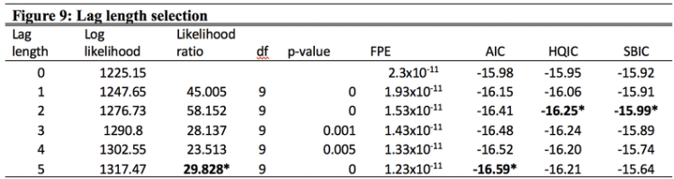
The next column shows the output from the Final Prediction Error test (FPE). This test examines which model lag length minimizes the predicted error while weighting different models by their degrees of freedom. The result of the test suggests five lags should be included in the model (Stata manual, 2011). The final three columns of Figure 9 are the results of the Akaike, Hannan-Quinn, and Scharz/Bayesian information criterions. These tests evaluate models of different lag length by their goodness of fit while penalizing over-parameterized models.
These tests suggest using the lag length which corresponds to the minimum test statistic value. Figure 9 shows that the Akaike recommends five lags while the other two tests suggest using a lag length of 2. Given that a lag length of 2 months is not sufficient address the autocorrelation present in these series these latter recommendations were ruled out and a lag length of 5 was chosen due to the consensus of the tests.
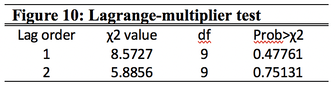
Figure 10 is the Lagrange-multiplier test which evaluates the autocorrelation at the first and second lag order post-estimation at both lag orders at any standard level of significance. This suggests that the model is successfully capturing the relevant dynamics of the data. As stated previously, more parsimonious models with fewer lags displayed significant autocorrelation which in turn suggested a lag length of 5.
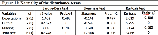
The Jarque-Bera test in Figure 11 was conducted to evaluate the disturbance terms in the primary model. The results show that both the expectations and leading indicator fail to reject the null hypothesis of a normally distributed disturbance while output growth strongly rejects the null hypothesis. This test is not constructive; it does not suggest possible remedies for the non-normal distribution of the output growth shock. Both skewness and kurtosis tests are displayed in Figure 15, they suggest that the non-normality of the output shock is coming from significant kurtosis. The consequence of this test is that, for output growth, in ‘n’ number of shocks we cannot say that 66% of them will be within one standard deviation. Reassuringly, the main shock of interest is the expectations shock which seems to be behaving correctly.[1]
VII. Conclusion
There are two main questions that this paper sought to address, both of which are related to expectations in the Canadian economy. The first question dealt with how prediction can moderate the business cycle. The idea behind this comes from the RBC literature on news shocks and has ramifications for economics as a discipline. If it is true that prediction moderates the business cycle then studying the economy and developing better forecasting could have large welfare effects. The results of this paper suggest that the increasingly precise forecasts of economic variables do not explain moderation especially in light of the increase in output variance following the 2008 financial crisis.
The other major vein of this paper focused on determining whether unexplainable pessimism or optimism has any economically significant effects. Unlike past literature, the three VAR models of this paper consistently found that these so called animal spirits are not having a large impact on the economy. This result suggests that expectations should still be thought about in the neo-classical context where expectations are simply an aggregation of the information available to agents, who are making their best guess about the future.
The policy implications of this paper are not immediately obvious. Policy makers cannot encourage baseless economic optimism to improve the economy. But from a wider methodological standpoint this paper suggests that using rational agents and micro-based models are appropriate approximations of the real world macro-economy. This work is necessary to confirm that the modeling done for policy evaluation rests on firm empirical regularities.
VIII. Appendix
[1] The same tests were done on the secondary VAR models and the same procedure was used in evaluating their robustness
References
Bank of Canada. Business outlook survey. (2013, May 6). Retrieved from
http://www.bankofcanada.ca/stats/bos/quarter/spring_2013
Barksky, R. & Sims, E. (2010). Information, animal spirits, and the meaning of innovations in
consumer confidence. NBER working paper series, 15049.
Diamond, P. (1982). Aggregate Demand Management in Search Equilibrium.
Journal of Political Economy, 90(5), 881-894
Gergen, Kenneth. (1982). Toward transformation in social knowledge.
New York: Springer-Verlag, Page 45-49
Greenwood, J. & Hercowitz, Z. & Krusell, P., (1992). Macroeconomic implications of
investment-specific technological change. Federal Reserve Bank of Minneapolis.
Grisse, C.(2008). Are expectations about economic activity self-fulfilling? An empirical test.
Federal Reserve Bank of New York. December, 2008.
Jiamovich, N. & Rebelo, S. (2009). Can news about the future drive the business cycle?
American Economic Review, 99(4), 1097-1118
Leenders, M. (2013, May 13). About the Ivey purchasing
managers index. Retrieved from: http://www.iveypmi.ca/english/about/index.htm
Lucas, R. (1976). Econometric policy evaluation: A critique.
Carnegie-Rochester Conference Series on Public Policy, 1(1), 19-46
Mathworks (2010). Matlab manual. 7(12). http://www.mathworks.com/help/toolbox/ident/ug/bq5z7kv.html
Simon, J. (2000). The long boom. Essays in Empirical Macroeconomics.
Phd Dissertation, Chapter 1
Sims, C. (1980). Macroeconomics and reality. Econometrica, 48(1), 1-48
Sims, C. (1992). Interpreting the macroeconomic time series facts. European Economic Review,
36, 975-1011.
Schmitt-Grohe, S. & Uribe, M. (2012). What’s news in business cycles.
Econometrica, 80(6)
Stata quick reference and index, (12) 2011, Stata Press: College Station, TX
Statistics Canada. (2012, May 23). Canadian composite leading indicator. Retrieved from:
http://www23.statcan.gc.ca/imdb/p2SV.pl?Function=getSurvey&SDDS=1601&Item_Id=1071&lang=en
Stock, J. & Watson, M. (2003). Has the business cycle changed and why?. NBER
Macroeconomics Annual 2002, 17, Retrieved from http://www.nber.org/chapters/c11075
Rogobon, R. (2003). Identification through heteroskedasticity.
The Review of Economics and Statistics. 85(4), 777-792.
Vogelvang, B. (2005). Econometrics: Theory and applications.
Harrow, England: Prentice Hall
