
Keenan Viney
Introduction
The Great Depression happened at a time when relatively little was understood about the interface between financial markets and the macro-economy functioned. The result was a poor monetary policy response which served to prolong and deepen the downturn.
Bernanke’s (2004) speech highlights that central bankers paradoxically constricted the money supply and politicians raised import tariffs. This disastrous outcome of this response fuelled the desire to better understand the functioning of the macro-economy and avert large welfare losses.
The major recession in 2008 came at a time when central bankers knew far more about how the economy functioned. Of course, monetary policy was being conducted in a different way, and this crisis served to test the ability of central bankers to stabilize the macro-economy. This paper will track some of the lesser known events associated with monetary policy before and during the crisis. By using an augmented IS-AS model it is possible to track some of the lesser known facets of monetary response to the 2008 financial crisis. From the bungled anticipation of the crisis, the limits of low inflation monetary intervention, and the Taylor-rules which minimizes social loss. These three lesser known aspects of the 2008 recession can be explored using a Neo-Wicksellian model proposed by Weise (2007).
In 2006, the United States Treasury bond yield curve was flat. The shape of the yield curve is often used as a leading indicator and a flat yield curve is an ominous sign. However, speaking at the Economic Club of New York, Ben Bernanke (2006) argued that the yield curve being observed was the result of a particular term structure. Under normal circumstances, investors require a greater return on long-term bonds as opposed to short term bonds because they have a greater interest rate and inflation risk associated with them. If inflation and interest rates become less volatile then the term premium demanded by investors would fall. This is precisely what Bernanke thought was occurring. Driven by better monetary policy with greater transparency, developed countries were seeing term premiums fall as expected by this line of reasoning. Because a decrease in the term premium would have a stimulatory effect (through lowering of realized interest rates) the Federal Reserve should raise interest rates. This means that the effective monetary tightening coincided with the crash in 2008. Thus the Federal Reserve failed to dampen a crisis by convincing themselves that the “yield curve has new fundamentals” (2006).
Low inflation monetary policy showed its weakness during the crisis as well. There was a widespread realization of the dynamic inconsistency problem in which nominal interest rates could not decrease below zero. This was evident in the widespread use of fiscal policy which is generally eschewed by top economists. Unfortunately, governments cannot run deficits forever. As governmental budget constrains bit, central banks had to use other tools in order to manage the economy. One such technique was shown by Operation Twist in 2011. The Federal Reserve sold short on short-term bonds and brought long-term Treasury bonds (Harding, 2011). This maintained the high powered money on the Federal Reserve’s balance sheet and rotated the term structure downward. By doing this the Federal Reserve was trying to convince agents that inflation will not spike in the next few years. This term structure rotation also signals that monetary policy will have more persistence thus making monetary policy more effective for a given change in the federal funds rate.
One facet of Federal Reserve operation that is often overlooked is its lack of an explicit inflation target. United States policy is in contrast to other countries like Canada, Australia, and New Zealand that have central banks committed to maintaining a certain band of inflation regardless of the consequences for output. The advantage of explicit rules is that agents are not constantly trying to guess what the central bank will do next, as they are in the United States. However, without an explicit inflation target the Federal Reserve is able to stimulate output. The Neo-Wicksellian model used in this paper allows the direct comparison of different monetary policy rules for different economic shocks, especially those that relate to the recession of 2008.
Economic Model
In practice monetary policy is much more difficult than its simple portrayal in the Neo-Wicksellian model. That said, the IS-LM and the AS-AD model have been a reliable way to think about the general effects of various macroeconomic shocks. The Neo-Wicksellian model devised by Weise (2007), augments the price-output and interest rate-output spaces with a model of the term structure. This allows for a clearer understanding of the way monetary policy functions in the real world while exposing more of the real world limitations that central banks face.
The Neo-Wicksellian model can be characterized by four equations. The model is recursive in that an exogenous shock is transmitted from the term structure to the money market (IS curve) through to the medium run price-output space of the aggregate supply curve. A Taylor rule type monetary policy reaction function is then added to determine the federal funds rate which enters into the term structure. To better understand the relationships between variables let us consider each equation in turn.
The term structure equation is specified as follows:
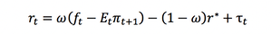
where ft is the federal funds rate which is set by the central bank in minimizing its social loss function. In the real world, this rate is set in the overnight bank lending market. The Federal Reserve effectively has control of the one month Treasury bill rate through the overnight bank lending rate. The variable r* is the natural real rate of interest, it is exogenous to the model and can be shocked by changes to productivity growth or the national savings rate. The natural real rate of interest will often decrease before a recession because lower productivity growth is expected. The variable ω can rotate the term structure and represents the policy persistence of the federal funds rate. Weise (2007) specifies ω=0.25 from empirical work but this exogenous variable is to some extent controlled by the central bank as in the case of Operation Twist. The Et∏t+1 term used by Weise uses an expectation operator to show the market forming adaptive expectations such that Et∏t+1 = ∏t. Finally, the variable tau is an exogenous shifter of the term structure. In Bernanke’s 2006 speech, he suggested that there had been a negative term structure shock as the result of a flight to quality.
The next equation is for the Investment-Savings (IS) curve which is represented in interest rate-output space. The equation is specified as follows:

The variable α states the slope of the IS curve[1]. The variable r* is that natural real rate of interest, and also appears in the term structure equation. The ut variable is an exogenous demand shock, which would occur if there is a tax decrease for example. Importantly, rt is determined by the term structure equation and it is through this mechanism that the federal funds rate shift the IS curve.
The aggregate supply relationship is in price level-output space and is specified as follows:
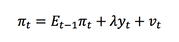
As in the term structure equation, the expected inflation is formed adaptively so that Et-1∏t = ∏t-1. The variable vt is an exogenous price shock which could be the result of a large change in the price of oil, for instance. The variable yt comes from the IS equation and is multiplied by λ. The full aggregate supply relation used in this Neo-Wicksellian model is similar to the Lucas supply curve but without forward looking expectations for simplicities sake.
The final equation used in this model differs from Weise’s more pedagogical model. Rather than using the monetary policy reaction function (MPRF) specification of Weise[2], this paper uses the more widely recognized Taylor-rule:
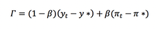
This is a social loss function which the central bank seeks to minimize by adjusting the federal funds rate. Furthermore, it allows for different weights to be placed on the output and inflation gap which reflects different central bank preferences over output and inflation. This will allow for social loss to be compared for different central bank preferences β.
Computational Model
This paper utilizes GAMS to simulated the Neo-Wicksellian model and gain some insight into the lesser known central bank policies that influenced the 2008 financial crisis. GAMS allowed for relatively easy imputation of equations from the Weiss paper. By programming a loop into the output script, the results in each period could be collected and impulse response functions could be graphed. These visualizations are very helpful in thinking about the effect and response to different economic shocks. When this model is solved by hand impulse response functions can be graphed but would be approximations and may not capture the actual magnitude of changes.
One key advantage of using GAMS for this model was the freedom in setting a monetary policy rule. In the Weiss paper, he specifies a particular Taylor-rule which presumes that the Federal Reserve simply tries to minimize the inflation gap. By adding a slope coefficient, it is possible to show a stabilizing monetary policy rule when solving by hand. While this decision makes some sense for teaching the model to students, it is too limited when exploring central bank policy. Since the Federal Reserve does not have an explicit inflation target, there is the possibility to trade off some inflation for additional output. The model specified in GAMS not only allows for this more complex Taylor-rule to be implemented, but also permits experiments to be done on the consequences of central bank preferences.
Scripts programmed in GAMS tend to be fairly transparent especially if there is extensive commenting, nevertheless what follows is a description of the script. After the title of the script the solver is specified. MINOS was used and worked for all of the experimental specifications with very low computational cost.
The next section specified the scalar values of the model which were chosen either by the empirical recommendation of the Weise (2007) article or if there was no recommendation; by choosing a reasonable value for the time period in which experiments will take place. The next section specifies the different exogenous shocks that can perturb this model: demand, price, term structure, and real natural interest rate shocks. The shocks are then parameterized and it is in this section that shocks of different magnitude are specified. The ‘Computation and Equation’ section specifies all of the endogenous variables in the model and the equations that relate them. It should be noted that equation 5 states that the central bank should minimized the sum of social loss in all periods. Finally, initial values are set, the solve function is specified, and a loop is created to give easily interpretable results.
Experiments
This paper will conduct experiments to examine three facets of Federal Reserve policy in relation to the 2008 financial crisis. Generally, it is the direction rather than the magnitude of results that we are interested in. However, when different shocks are applied, every effort is made to insure that they are of comparable size. All of the experiments will be done ceteris paribus in order not to confound the results.
Experiment 1 compares the Federal Reserve response to a term structure shock or to a decrease in the natural rate of interest due to an anticipated slowdown in growth. This is similar to the dilemma that Bernanke faced in 2006 with the observed flat yield curve. By comparing the federal funds rate in these two cases it is possible to infer the consequences of deciding that the flat yield curve was the result of a negative term structure shock caused by a ‘flight to quality’ by foreign investors.
Experiment 2 shows the effect of a change in the policy persistence variable ω. This is analogous the Federal Reserve’s Operation Twist in late 2011. By short-selling short-term bonds and buying long-term bonds, the Federal Reserve was trying to signal that the contemporary low interest rates would continue while inflation would be held in check. It will be interesting to note how changes to the federal funds rate will be altered in magnitude by this exogenous change in policy persistence.
Finally, Experiment 3 will test the importance of the Federal Reserves’ preference in regards to the output and inflation gap on social loss. This test is valid for the United States because there is no firm inflation target that constrains the central bank. That means that the Federal Reserve has the ability to hold interest rates low, and while inflation would increase but output would be stimulated. The without a commitment to some specific Taylor-rule, the social loss due to various shocks is expected to differ.
Results
Experiment 1
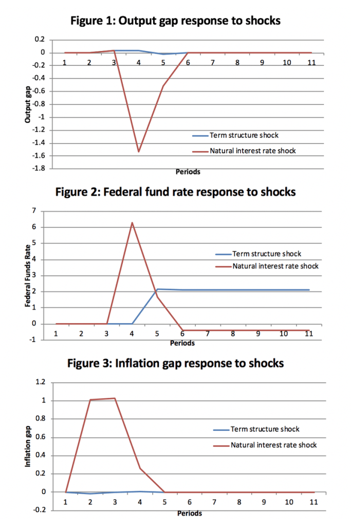
These graphs show the differences in impulse response to a term structure shock versus natural real rate of interest shock. This is analogous to the mistake by Bernanke in 2006 when he interpreted the flat yield curve as a negative term structure shock as opposed to a reduction in the natural rate of interest.
Figure 1 shows the output gap response from these two possible shocks. Interestingly, even though these shocks are of the same magnitude the natural interest rate shock has a far greater effect on output than a term structure shock. Figure 3 is the same story, in that the term structure shock has a very small effect. Figure 2 shows the federal funds rates that are optimal in response to both of these shocks. What is interesting here is long run change, which shows that for a term structure shock the federal funds rate should be raised. For a shock in the natural rate of interest the federal funds rate should be held very low in order to stimulate the economy. By assuming that the flat yield curve in 2006 was the result of a term structure shock, the Federal Reserve was following precisely the wrong policy. In 2008 it became obvious that productivity growth had decreased and along with it the natural interest rate, the Federal Reserve was running tight monetary policy when their policy should have been stimulatory.
Experiment 2
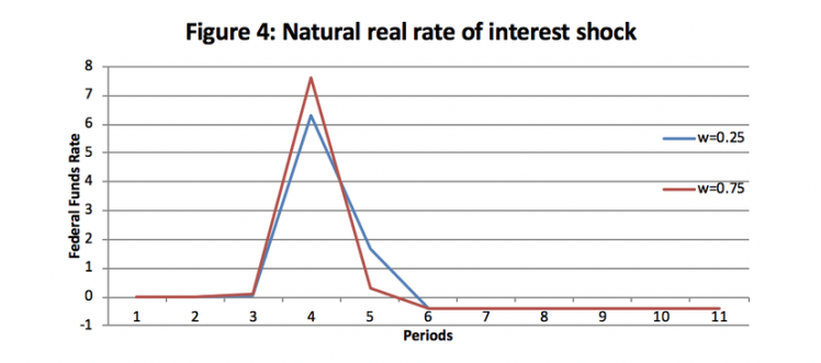
These three figures show the optimal federal funds rate response to three different shocks. There are two treatments on the policy persistence term which adjusts the slope of the term structure curve. This is analogous to Operation Twist in which the Federal Reserve bought and sold bonds of different maturities to alter the term structure, essentially increasing the ω variable.
Figure 4 shows a surprising result in that optimal monetary policy in response to a real interest rate shock is not particularly sensitive to policy persistence. This may be due to the inertia of adaptive expectations that are important to how real interest rate shocks are transmitted in this system.
Reassuringly, Figure 5 and 6 show that as monetary policy becomes more persistent smaller changes in the federal funds rate are possible for equivalent effects. This result suggests that because the Federal Reserve was maintaining federal funds rates at very low levels, the only way to further stimulate the economy was through changing policy persistence. From the somewhat counter intuitive result that real interest rate shocks are insensitive to changes in policy persistence it is also possible to infer something about Federal Reserve expectations. The three results together suggest that the Federal Reserve is assuming that price and demand shocks will be important in the medium term while real interest rates will be relatively stable.
Experiment 3

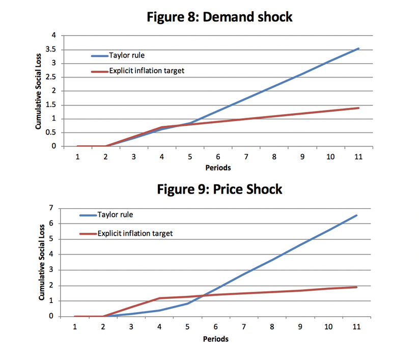
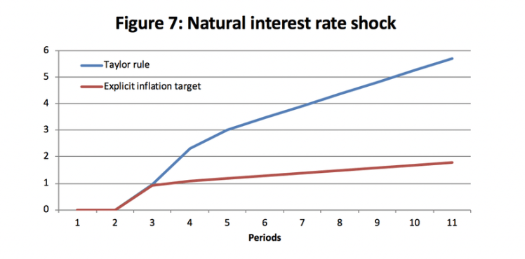
This experiment compares the social loss that results from different monetary policy rules across different shocks. Figure 7 shows that the social loss resulting from a natural real interest rate shock is higher under a Taylor rule specification. This means that when the central bank tries to minimize a linear combination of output and inflation (β=0.5), they end up inflicting more social loss than they would have if they simply minimize inflation. The same result is evident in both Figure 8 and 9. The explicit inflation target (β=1) mitigates loss under every shock. This experiment is interesting because it highlights the differences between Federal Reserve policy and the policy of other central banks. While the Federal Reserve follows some approximation of the Taylor-rule, many other central banks focus on minimizing the inflationary gap. Finding this result is not especially surprising since it is a well established theme in central banking literature. But this result is often derived out of more complicated models with rational expectations and stochastic elements. So it is interesting that explicit inflation targeting is superior in this relatively simple model with adaptive expectations.
Discussion
This Neo-Wicksellian model is limited in that it does not include rational expectation and it is vastly simpler than the actual macro-economy. Despite the lack of rational expectation, Experiment 3 showed that this model suggests similar conclusions about optimal monetary policy as more complex models.
Adaptive expectations remain part of many simple models in macro economics because the equations are much easier to work with but further work with this model should attempt to include more reasonable forward-looking rational expectations. This model is also very simplistic closed economy without important real world factors such as a labour or financial market. Specifying such a simple model is in some ways beneficial since, like the IS-LM model, it allows us to think about a very complex system and get some useful results. Another advantage to the simplicity of this model is that it is easy to include more complexity. This model differs from Weise’s (2007) specification in that it includes a more complicated monetary policy reaction function which is important for thinking about central bank policy.
This paper has explored three lesser known aspects of Federal Reserve policy in the context of the 2008 financial crisis. Experiment 1 showed that by misinterpreting the cause of the flat yield curve in 2006, the Federal Reserve implemented tight monetary policy when it should have been expansionary. Had the interpretation of the flat yield curve been taken as a pessimistic omen (as it usually is), the Federal Reserve would have been in a better position to respond to the 2008 recession, especially in light of the lags associated with monetary policy effectiveness. Of course this model does not say conclusively that a real interest rate decrease rather than a term structure shock was causing the flat yield curve. But it suggests caution when setting monetary policy in contrary to the information conveyed by well accepted leading indicators.
Experiment 2 explored the consequences of Operation Twist in late 2011. By shorting short-term bonds and buying long-term bonds the Federal Reserve altered the slope of the term structure and signalled greater policy persistence. The findings of this paper show that this action by the Federal Reserve means that a change in the interest rate of a given magnitude will become more effective under this policy. Generally, central banks do not want particularly sensitive policy instruments because it can lead to overshooting output and inflation targets. At extremely low interest rates and low growth levels the Federal Reserve needs what little interest rate variation it has to be more effective. Operation Twist and other programs like it are important tools for central banks facing large recessions in a low inflation era.
The most general conclusion of this paper came from Experiment 3. The current policy of the Federal Reserve which minimizes both the output gap and inflation serves to increase the social loss. Other countries like Canada, Australia, and New Zealand use explicit inflation targets which are shown in this paper to be more socially effective. This suggests that the Federal Reserve should stop trying to manage output and should set an implicit inflation rate. As with the other two experiments, this paper suggests tools and methods which can improve how central banks function. This paper began by discussing how the Great Depression spurred an exponential growth in our knowledge about central banking. The 2008 financial crisis is an opportunity for another great leap forward in macroeconomic knowledge.[1] ‘α’ can be derived from the Keynesian income-expenditure model.
[2]yt = -β(∏t – ∏)
Appendix – GAMS Code*TITLE: Neo-Wicksellian Model
*Created by Keenan Viney
OPTION NLP=MINOS
************************************
*Defining scalar parameters
************************************
SCALARS
w
*rstar persistence of central bank policy /0.25/
*finitial natural rate of interest /0.05/
a federal funds rate /0.05/
lambda IS curve slope /1/
beta AS output sensitivity /0.5/
ystar natural output level /1/
pistar base inflation /0.10/
************************************
*Define the time horizon
************************************
SETS T EXTENED HORIZON /0*24/
T0(T) PERIOD ZERO
T1(T) PERIOD ONE ;
T0(T) = YES$(ORD(T) EQ 1);
T1(T) = YES$(ORD(T) EQ 1);
DISPLAY T0, T1;
display T;
************************************
*Possible system shocks
************************************
parameters
* Definition of policy shocks in percentage (0 to 1) changes
uper(T) Demand shock(in % change)
vper(T) Price shock(in % change)
rstarper(T) Natural interest rate shock(in % change)
tauper(T) Liquidity shock (in % change)
* Definition of exogenous variables (in levels)
u(T) Demand shock (in levels)
v(T) Price shock (in levels)
rstar(T) Natural interest rate shock (in levels)
tau(T) Liquidity shock (in levels);
* Definition values for policy shocks
uper(T) = 0.0 ; vper(T) = 0.0 ; rstarper(T) = 0.00 ; tauper(T) = 0.00 ;
* Base values for exogenous variables
u(T) = 0 ; v(T) = 0 ; rstar(T) = 0.05 ; tau(T) = 0 ;
************************************
*Shock parameters
************************************
SETS
TS1(T) all periods /4*24/;
* Demand shock
uper(TS1) = 0.00;
* Price shock
vper(TS1) = 0.50;
* Natural interest rate shock
rstar(TS1) = 0.00;
* Term structure shock
tauper(TS1) = 0.00;
* Shock applications (commented out in a default run)
u(TS1) = uper(TS1) ;
v(TS1) = vper(TS1) ;
rstar(TS1) = rstarper(TS1);
tau(TS1) = tauper(TS1);
* reporting poicy and exogenous variable values
PARAMETER REPORTEX POLICY AND EXOGENOUS VARIABLES VALUES;
REPORTEX(T,”Demand shock”) = u(T);
REPORTEX(T,”Price shock”) = u(T);
REPORTEX(T,”Natural interest rate”) = u(T);
REPORTEX(T,”Term structure shock”) = u(T);
************************************
*Computation and Equations
************************************
Variables
y(T) output
f(T) federal fends rate
r(T) real interest rate
pi(T) inflation rate
gamma(T) social loss function
obj objective function
EQUATIONS
eq1(T) Term structure curve (TS)
eq2(T) Investment-Savings curve (IS)
eq3(T) Aggregate supply curve (AS)
eq4(T) Social loss function
eq5 Federal funds rate non-zero constraint
eq6 Objective function;
eq1(t+2).. r(t+2) =E= w*(f(t+2) – pistar) +(1-w)*rstar(t+2) + tau(t+2) ;
eq2(t+2).. y(t+2) =E= -a*(r(t+2) – rstar(t+2)) +u(t+2) ;
eq3(t+2).. pi(t+2) =E= pi(t+2) + lambda*y(t+2) + v(t+2) ;
eq4(t+2).. gamma(t+2) =E= (1-beta)*(y(t+2) – ystar) – beta*(pi(t+2) – pistar)
eq5.. sum (t, f(t+2)) =g= 0;
eq6.. obj =E= sum (t, gamma(t+2));
************************************
*Setting initial values
************************************
f.L(T) = 0.00 ; y.L(T+2) = 1 ; pi.L(T+2) = 0.03 ;
r.L(T+2) = 0.02 ; gamma.L(T) = 0;
*fixing initial steady-state values for lagged endogenous variables
pi.FX(TS1) = 0 ;
MODEL NONLDYN /eq1, eq2, eq3, eq4, eq5, eq6 / ;
SOLVE NONLDYN MINIMIZING obj USING NLP;
* Reporting solution values
PARAMETER REPORTS SOLUTION VALUES IN LEVELS;
REPORTS(T,”GDP”) = y.L(T);
REPORTS(T,”Inflation”) = pi.L(T);
REPORTS(T,”Fed funds rate”) = f.L(T);
REPORTS(T,”Real interest rate”) = r.L(T);
REPORTS(T,”Social Loss”) = gamma.L(T);
* Showing final results
DISPLAY REPORTEX;
DISPLAY REPORTS;
* Write to File
* Define the file: change this name for different experiments
file neowicksellian /neowicksellian01.txt/;
* Make the current file
put neowicksellian;
* Write periods to file
put ‘t’; loop(t, put ‘,’, put t.t1); put /;
* Write variable to file
put ‘y’; loop(t, put ‘,’, put y.l(t)); put /;
put ‘pi’; loop(t, put ‘,’, put pi.l(t)); put /;
put ‘f’; loop(t, put ‘,’, put f.l(t)); put /;
put ‘r’; loop(t, put ‘,’, put r.l(t)); put /;
put ‘gamma’; loop(t, put ‘,’, put gamma.l(t)); put /;
* Close the file
putclose NeoWicksellian;
References
Bernanke, Ben. “Money, Gold, and the Great Depression” Lexington, Virginia,
At the H. Parker Willis Lecture in Economic Policy, Washington and Lee
University. March 2, 2004.
Bernanke, Ben. “Reflections on the Yield Curve and Monetary Policy” New York, New York,
At the Economic Club of New York, March 20, 2006
Harding, R. (2011, September 21). Fed launches $400bn ‘operation twist’.
Financial Times. Retrieved from http://www.ft.com/cms/s/0/3deaf5fc-e478-11e0-92a3-00144feabdc0.html
Weise, Charles (2007) “A Simple Wicksellian Macroeconomic Model,” The B.E. Journal of
Macroeconomics: Vol. 7: Iss. 1 (Topics), Article 11.
